Kalman Filter of Continuous Systems Using Matlab Ppt

Introduction to Kalman Filter Matlab

MATLAB provides a variety of functionalities with real-life implications. This article covers a very important MATLAB functionality called the 'Kalman filter. We use Kalman filter to estimate the state of a given system from the measured data. Once this is done, refinement of estimates is also done. Let's first understand what the Kalman filter is.

What is Kalman Filter?

Kalman filter developed primarily by the Hungry-based Engineer, Mr. Rudolf Kalman, is an algorithm used to estimate state of a given system using measured data. The Kalman filter's algorithm is a 2-step process. In the first step, the state of the system is predicted and in the second step, estimates of the system state are refined using noisy measurements. Kalman filter has evolved a lot over time and now its several variants are available. Kalman filters are used in applications that involve estimations, like computer vision, navigation&guidance systems, signal processing, and econometrics.

Guidance, Navigation & Control

Kalman filters are used in guidance, navigation, and control systems. These filters synthesize position & velocity signals in sensor fusion. This is achieved by fusing together GPS & IMU measurements (inertial measurement units). Kalman filters are commonly used in estimating the value of a signal which cannot be measured. For example, the temperature inside the aircraft engine or turbine, as temperature sensors would fail in such conditions. These filters are also used commonly along with LQR compensators (linear-quadratic-regulator) for LQG control(linear-quadratic-Gaussian).

Now that we have refreshed our understanding of Kalman filtering, let's see a detailed example to understand Kalman filter in MATLAB

Steps to Implement Kalman Filter in Matlab

Below are the steps user will need to follow to implement Kalman filter in MATLAB. The MATLAB code is also provided along with the steps:

1. We will define length of simulation:

simulen = 30

2. Let us now define the system

b = 1 c = 4

(we use b = 1 for constant systems; you can use |b| < 1 for a system of 1^st order)

3. Next, we will declare the covariances of noise

Q=0.02; R=3;

4. We will now pre-allocate the memory for the arrays. Please keep in mind that doing pre-allocation is not necessary, we only do it to speed-up the processing in MATLAB.

x=zeros(1,nlen); z=zeros(1,nlen);

5. Next, we will define initial estimates for 'the state' and error ('priori error')

inpriori=zeros(1,nlen); inposteriori=zeros(1,nlen); residual=zeros(1,nlen); rapriori=ones(1,nlen); raposteriori=ones(1,nlen); k=zeros(1,nlen);

6. Next, we will compute the process noise and measurement noise

w=randn(1, nlen); v1=randn(1,nlen);w=w1*sqrt(Q); v=v1*sqrt(R);

Here we are taking percentage for a better comparison

7. Let's now define initial condition on x and initial estimates for posteriori covariance and state

x_0= 2.0; inposteriori_0=1.5; raposteriori_0=1;

8. Next, we will compute the first guesses of all the values. This will be done based on the initial estimates of state followed by posteriori covariance. Next steps will be computed in loopComputing state & output:

x(1)= b *x_0+w(1); z(1)= c *x(1)+v(1);

Our Predictor equations are:

inpriori(1)= b*inposteriori_0; residual(1)=z(1) – c *inpriori(1); rapriori(1)= b*b*raposteriori_0+Q;

Corrector equations will be:

k(1)= c *rapriori(1)/ (c * c *rapriori(1)+R); raposteriori(1)=rapriori(1)*(1 – h*k(1)); inposteriori(1)=inpriori(1)+k(1)*residual(1);

Computing rest values:

for p =2:nlen, x(p) = b * x(p -1)+w(p); z(p) = c *x(p)+v(p); inpriori(p)= b *inposteriori(p-1); residual(p)=z(p) – c *inpriori(p); rapriori(p)= b * b *raposteriori(p -1)+Q; k(p)= c *rapriori(p)/(c * c *rapriori(p)+R); raposteriori(p)=rapriori(p)*(1 – c *k(p)); inposteriori(p)=inpriori(p)+k(p)* residual(p); end p =1:nlen;

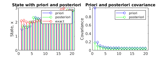
9. Let's now plot state & their estimates

subplot(221); h1=stem(p +0.25,inpriori,'b'); hold on h2= stem(p +0.5,inposteriori,'g'); h3=stem(p,x,'r'); hold offlegend([h1(1) h2(1) h3(1)], 'priori', 'posteriori','exact'); title('State with priori and posteriori'); ylabel('State, x'); xlim=[0 length(p)+1]; set(gca,'XLim',xlim);

10. Let us also plot the covariance

subplot(222); h1= stem(p,rapriori,'b'); hold on; h2=stem(p,raposteriori,'g'); hold off legend([h1(1) h2(1)], 'priori', 'posteriori'); title('Priori and posteriori covariance'); ylabel('Covariance'); set(gca,'XLim',xlim);

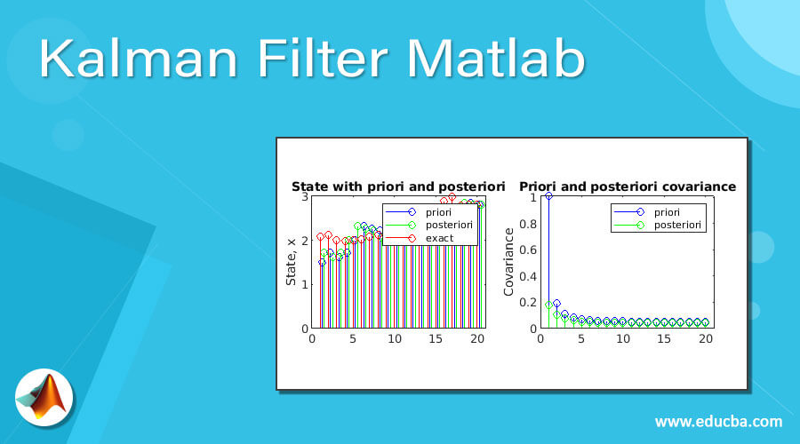
On implementing above code, below is how our output will look like in MATLAB:

Conclusion

Kalman filters are perfect for systems that are changing continuously. These filters have the advantage of being light on the memory as they don't require to keep anything in history other than their previous state. Kalman filters are also very fast which make them great tool for embedded systems and real-time problems.